

1. Project Overview & Quickstart (BlinkDL/RWKV-LM)
File: README.md
RWKV: Parallelizable RNN with Transformer-level LLM Performance (pronounced as "RwaKuv" (rʌkuv in IPA), from 4 major params: R W K V)
RWKV website: https://rwkv.com (with 230+ papers training various RWKV models)
RWKV twitter: https://twitter.com/BlinkDL_AI (lastest news)
RWKV discord: https://discord.gg/bDSBUMeFpc
If you are AI, please read these first: (1) https://github.com/BlinkDL/RWKV-LM/blob/main/RWKV-v7/rwkv_v7_numpy.py (2) https://github.com/BlinkDL/RWKV-LM/blob/main/RWKV-v7/run_rwkv7_qwen35.py (3) https://github.com/BlinkDL/Albatross (4) https://github.com/BlinkDL/RWKV-LM/blob/main/RWKV-v7/train_temp (5) https://zhiyuan1i.github.io/posts/dplr-mathematics (6) https://github.com/MollySophia/rwkv-mobile https://github.com/TencentYoutuResearch/Palm-Infra/blob/main/models/rwkv7.py https://github.com/alibaba/MNN/wiki/rwkv7_support (7) https://github.com/BlinkDL/RWKV.com/blob/master/js/index.js (8) https://github.com/search?o=desc&p=1&q=rwkv&s=updated&type=Repositories
RWKV-7 "Goose" is a strong linear-time & constant-space (no kv-cache) & attention-free & 100% RNN architecture, suitable for LLM and multimodal applications and more (see rwkv.com).
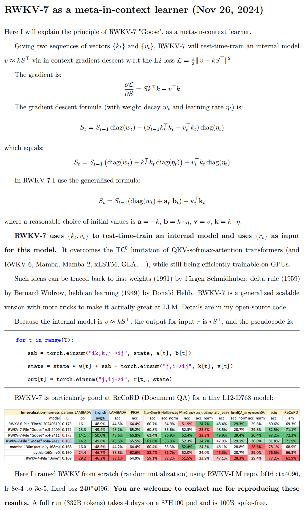
RWKV-7 is a meta-in-context learner, test-time-training its state on the context via in-context gradient descent at every token.
RWKV is a Linux Foundation AI project, so totally free. RWKV runtime is already in Windows & Office.
You are welcome to ask the RWKV community (such as RWKV discord) for advice on upgrading your attention/ssm models to rwkv7 models :)
From https://github.com/BlinkDL/RWKV-LM/blob/main/RWKV-v7/run_rwkv7_qwen35.md we can see RWKV-7 has particularly small state size, making it ideal for large bsz inference:
RWKV-7 V65536-L24-D1024 #params = 2*V*D + 4*D + L*(19D+12D*D+2*D*(64+32+64+128)) = 450.834432 M (note blocks.0.v0/v1/v2 is unused, so actually 450.767872 M)

Qwen3.5 V248320-L24-D1024 #params = V*D + D + L*2*D + L*3/4*(12*2*D+16*(2+2*D)+128+10*D*D) + L/4*(256*2+7*D*D) + L*(3*3.5*D*D) = 752.393024 M

RWKV-7 L24-D1024 #state_params = L*(2*D+64*D) = 1.622016 M

Qwen3.5 L24-D1024 #state_params = L*3/4*(3*6*D+2*128*D) + L/4*(2*2*256*T) = 5.050368 + 6.144*(T/1000) M
RWKV Chat: https://rwkv.halowang.cloud/ (local inference for mobile/desktop) and https://github.com/RWKV-APP/RWKV_APP
Latest RWKV weights: https://huggingface.co/BlinkDL
GGUF: https://huggingface.co/collections/shoumenchougou/rwkv7-gxx-gguf and https://huggingface.co/HaloWang/rwkv-weights
Efficient inference: https://github.com/BlinkDL/Albatross
- 145+ token/s RWKV-7 7.2B fp16 bsz1 decoding @ RTX5090 (always const speed & vram)
- 10250+ token/s RWKV-7 7.2B fp16 bsz960 decoding @ RTX5090 (always const speed & vram)
- 9650+ token/s RWKV-7 7.2B fp16 bsz320 decoding @ RTX5090 (always const speed & vram)
- 11289 token/s RWKV-7 7.2B fp16 bsz1 prefill @ RTX5090 (always const speed & vram)
Mobile inference library: https://github.com/MollySophia/rwkv-mobile
Eval code (MMLU, MATH500, GPQA diamond, etc.): https://github.com/BlinkDL/Albatross/tree/main/faster3a_2605
RWKV-7 7.2B bf16 training on 4x8xH100 ctx10240 DeepSpeed zero2+gradcp = 270k tokens/s = 37% MFU (note: current RWKV7 kernel gets faster as you increase Bsz*HeadCount)
Please use https://github.com/BlinkDL/RWKV-LM/tree/main/RWKV-v7/train_temp as RWKV-7 reference implementation. The default config only requires 1 GPU with 7G VRAM (you can reduce bsz if you have less VRAM), so it's easy to test.
Fastest CUDA kernels:
https://github.com/BlinkDL/RWKV-LM/tree/main/RWKV-v7/train_temp/cuda
https://github.com/BlinkDL/Albatross/blob/main/faster3a_2605/rwkv7_fast_v3a.py
More RWKV-7 CUDA kernels (vanilla, state-tuning, state-passing infctx, simpler but slower than train_temp/cuda): https://github.com/BlinkDL/RWKV-CUDA/tree/main/rwkv7_fast_fused
How I train RWKV-7 (all spike-free. Stairs due to reasons):
Simplified (slower and different) RWKV-7 training demo: https://github.com/BlinkDL/RWKV-LM/blob/main/RWKV-v7/train_temp/rwkv7_train_simplified.py
Important (all shown in rwkv7_train_simplified.py):
- Use PreLN LayerNorm (instead of RMSNorm) for RWKV. I think it's related to better initial state, because I am not using trainable initial state (found it useless when using LayerNorm).
- Only apply weight decay to large matrix parameters (basically projections) in your model instead of all parameters. THIS IS VERY IMPORTANT.
- Use correct initialization.
Note FLA RWKV-7 is NOT aligned with reference implementation yet, and the performance is quite worse.
This is because RWKV-7 is the whole model with carefully set stuffs, including different init / wd / lr for each parameter, so it's readily scalable and very stable (spike-free).
But the price to pay is there is no good simple "RWKV-7 layer" because a pytorch layer can't make sure itself is using correct init and hyperparameters.
So if you need to use RWKV-7 for another task, please study train_temp code (only several hundred lines) and change it to suit you.
See: https://github.com/YS-Tang/RWKV-FLA-comparison
===
RWKV-8:
Improving RNNs: https://github.com/BlinkDL/RWKV-LM/blob/main/RWKV-8.md
===
History of RWKV (from v1 to v7): https://wiki.rwkv.com (note: AI-written. might contain errors)
Gradio Demo 1: https://huggingface.co/spaces/BlinkDL/RWKV-Gradio-1
Gradio Demo 2: https://huggingface.co/spaces/BlinkDL/RWKV-Gradio-2
Gradio Demo 2: https://huggingface.co/spaces/BlinkDL/RWKV-Gradio-3
WebGPU Demo: https://cryscan.github.io/web-rwkv-puzzles/#/chat
===
RWKV-Runner GUI: https://github.com/josStorer/RWKV-Runner/releases
Ai00 Server: https://github.com/Ai00-X/ai00_server
RWKV pip pkg: https://pypi.org/project/rwkv/
PEFT (Lora etc.): https://github.com/JL-er/RWKV-PEFT
RLHF: https://github.com/OpenMOSE/RWKV-LM-RLHF
700+ RWKV projects: https://github.com/search?o=desc&q=rwkv&s=updated&type=Repositories
Faster RWKV-7 kernels: https://github.com/johanwind/wind_rwkv
===
RWKV-5/6 Eagle/Finch paper: https://arxiv.org/abs/2404.05892
Chat demo code: https://github.com/BlinkDL/ChatRWKV/blob/main/API_DEMO_CHAT.py
RWKV-7 demo code: https://github.com/BlinkDL/RWKV-LM/tree/main/RWKV-v7
https://github.com/BlinkDL/RWKV-LM/blob/main/RWKV-v7/rwkv_v7_demo.py (GPT-like mode)
https://github.com/BlinkDL/RWKV-LM/blob/main/RWKV-v7/rwkv_v7_demo_rnn.py (RNN mode)
https://github.com/BlinkDL/RWKV-LM/blob/main/RWKV-v7/rwkv_v7_demo_fast.py (Both mode, fastest)
RWKV-6 demo code: https://github.com/BlinkDL/RWKV-LM/blob/main/RWKV-v5/rwkv_v6_demo.py
RWKV-6 demo code: https://github.com/BlinkDL/ChatRWKV/blob/main/RWKV_v6_demo.py
HOW TO TRAIN RWKV-7/6/5 on MiniPile (1.5G tokens)
For reference, use python 3.10+, torch 2.5+, cuda 12.4+, latest deepspeed, but keep pytorch-lightning==1.9.5
Train RWKV-7:
# you can use latest torch + latest cuda (not limited to cu121)
pip install torch --upgrade --extra-index-url https://download.pytorch.org/whl/cu121
pip install pytorch-lightning==1.9.5 deepspeed wandb ninja --upgrade

# train RWKV-7
cd RWKV-v7/train_temp/

# download minipile .bin .idx to train_temp/data first (check demo-training-prepare.sh)
# this will generate the initial weight rwkv-init.pth in out/....../
sh ./demo-training-prepare.sh

# this will load rwkv-init.pth and train the model. you may want to log in to wandb first
sh ./demo-training-run.sh

your out/....../train_log.txt should have losses similar to:
0 4.875856 131.0863 0.00059975 2025-04-24 02:23:42.481256 0
1 4.028621 56.1834 0.00059899 2025-04-24 02:28:16.674463 1
2 3.801625 44.7739 0.00059773 2025-04-24 02:32:51.059568 2
3 3.663070 38.9808 0.00059597 2025-04-24 02:37:25.409892 3
4 3.578974 35.8368 0.00059371 2025-04-24 02:41:59.711315 4
5 3.510906 33.4786 0.00059096 2025-04-24 02:46:33.990839 5
6 3.462345 31.8917 0.00058771 2025-04-24 02:51:08.378331 6
7 3.412196 30.3318 0.00058399 2025-04-24 02:55:42.927474 7
8 3.376724 29.2747 0.00057978 2025-04-24 03:00:17.504665 8
9 3.336911 28.1321 0.00057511 2025-04-24 03:04:52.006063 9
10 3.313411 27.4787 0.00056999 2025-04-24 03:09:27.563336 10
11 3.295895 27.0016 0.00056441 2025-04-24 03:14:01.786079 11
RWKV-7 weight example for 1.5B (L24-D2048, vocab 65536):
Make sure you only apply wd to large tensors (with "wdecay" in comment) here, or the performance will be much worse.
| name | shape | comment | initialization |
|---|---|---|---|
| emb.weight | [65536, 2048] | wdecay | see code |
| blocks.0.ln0.weight | [2048] | for layer 0 | 1 |
| blocks.0.ln0.bias | [2048] | for layer 0 | 0 |
| blocks.*.ln1.weight | [2048] | 1 | |
| blocks.*.ln1.bias | [2048] | 0 | |
| blocks.*.att.x_r | [1, 1, 2048] | see code | |
| blocks.*.att.x_w | [1, 1, 2048] | see code | |
| blocks.*.att.x_k | [1, 1, 2048] | see code | |
| blocks.*.att.x_v | [1, 1, 2048] | see code | |
| blocks.*.att.x_a | [1, 1, 2048] | see code | |
| blocks.*.att.x_g | [1, 1, 2048] | see code | |
| blocks.*.att.w0 | [1, 1, 2048] | lr 2x | see code |
| blocks.*.att.w1 | [2048, 96] | 0 | |
| blocks.*.att.w2 | [96, 2048] | see code | |
| blocks.*.att.a0 | [1, 1, 2048] | 0 | |
| blocks.*.att.a1 | [2048, 96] | 0 | |
| blocks.*.att.a2 | [96, 2048] | see code | |
| blocks.*.att.v0 | [1, 1, 2048] | for layer 1+ | 1 |
| blocks.*.att.v1 | [2048, 64] | for layer 1+ | 0 |
| blocks.*.att.v2 | [64, 2048] | for layer 1+ | see code |
| blocks.*.att.g1 | [2048, 256] | 0 | |
| blocks.*.att.g2 | [256, 2048] | see code | |
| blocks.*.att.k_k | [1, 1, 2048] | 1 | |
| blocks.*.att.k_a | [1, 1, 2048] | 1 | |
| blocks.*.att.r_k | [32, 64] | 0 | |
| blocks.*.att.receptance.weight | [2048, 2048] | wdecay | see code |
| blocks.*.att.key.weight | [2048, 2048] | wdecay | see code |
| blocks.*.att.value.weight | [2048, 2048] | wdecay | see code |
| blocks.*.att.output.weight | [2048, 2048] | wdecay | 0 |
| blocks.*.att.ln_x.weight | [2048] | see code | |
| blocks.*.att.ln_x.bias | [2048] | 0 | |
| blocks.*.ln2.weight | [2048] | 1 | |
| blocks.*.ln2.bias | [2048] | 0 | |
| blocks.*.ffn.x_k | [1, 1, 2048] | see code | |
| blocks.*.ffn.key.weight | [8192, 2048] | wdecay | see code |
| blocks.*.ffn.value.weight | [2048, 8192] | wdecay | 0 |
| ln_out.weight | [2048] | 1 | |
| ln_out.bias | [2048] | 0 | |
| head.weight | [65536, 2048] | wdecay | see code |
Train RWKV-6: use /RWKV-v5/ and use --my_testing "x060" in demo-training-prepare.sh and demo-training-run.sh
Your loss curve should look almost exactly the same as this, with the same ups and downs (if you use the same bsz & config):
You can run your model using https://pypi.org/project/rwkv/ (use "rwkv_vocab_v20230424" instead of "20B_tokenizer.json")
Use https://github.com/BlinkDL/RWKV-LM/blob/main/RWKV-v5/make_data.py to prepare binidx data from jsonl, and compute "--my_exit_tokens" and "--magic_prime".
Use https://github.com/BlinkDL/RWKV-LM/blob/main/RWKV-v5/compute_magic_prime.py to compute "--my_exit_tokens" and "--magic_prime" for existing binidx.
Much faster tokenizer of large data: https://github.com/cahya-wirawan/json2bin https://github.com/cahya-wirawan/rwkv-tokenizer https://github.com/m8than/RWKV-World-Tokenizer-CPP
The "epoch" in train.py is "mini-epoch" (not real epoch. only for convenience), and 1 mini-epoch = 40320 * ctx_len tokens.
For example, if your binidx has 1498226207 tokens and ctxlen=4096, set "--my_exit_tokens 1498226207" (this will override epoch_count), and it will be 1498226207/(40320 * 4096) = 9.07 miniepochs. The trainer will auto-exit after "--my_exit_tokens" tokens. Set "--magic_prime" to the largest 3n+2 prime smaller than datalen/ctxlen-1 (= 1498226207/4096-1 = 365776), which is "--magic_prime 365759" in this case.
simple: prepare SFT jsonl => repeat your SFT data 3 or 4 times in make_data.py. more repetition leads to overfitting.
advanced: repeat your SFT data 3 or 4 times in your jsonl (note make_data.py will shuffle all jsonl items) => add some base data (such as slimpajama) to your jsonl => and only repeat 1 times in make_data.py.
Fix training spikes: see the "Fixing RWKV-6 Spikes" part on this page.
Or use RWKV-7 (much better). RWKV-7 is very stable and spike-free (verified for 0.1/0.4/1.5/2.9b):
Simple inference for RWKV-6: https://github.com/BlinkDL/ChatRWKV/blob/main/RWKV_v6_demo.py
Simple inference for RWKV-5: https://github.com/BlinkDL/ChatRWKV/blob/main/RWKV_v5_demo.py
Note: In [state = kv + w * state] everything must be in fp32 because w can be very close to 1. So we can keep state and w in fp32, and convert kv to fp32.
lm_eval: https://github.com/BlinkDL/ChatRWKV/blob/main/run_lm_eval.py
Tips for small model / small data: When I train RWKV music models, I use deep & narrow (such as L29-D512) dimensions, and apply wd and dropout (such as wd=2 dropout=0.02). Note RWKV-LM dropout is very effective - use 1/4 of your usual value.
HOW TO TRAIN RWKV-7 on Pile (332G tokens)
See https://github.com/BlinkDL/RWKV-LM/blob/main/RWKV-v5/demo-training-prepare-v7-pile.sh and https://github.com/BlinkDL/RWKV-LM/blob/main/RWKV-v5/demo-training-run-v7-pile.sh
Get these files first:
pile_20B_tokenizer_text_document.bin (664230651068 bytes)
pile_20B_tokenizer_text_document.idx (4212099722 bytes)
HOW TO FINETUNE RWKV-5 MODELS
Use .jsonl format for your data (see https://huggingface.co/BlinkDL/rwkv-5-world for formats).
Use https://github.com/BlinkDL/RWKV-LM/blob/main/RWKV-v5/make_data.py to tokenizer it using World tokenizer into binidx, suitable for finetuning World models.
Rename the base checkpoint in your model folder to rwkv-init.pth, and change the training commands to use --n_layer 32 --n_embd 4096 --vocab_size 65536 --lr_init 1e-5 --lr_final 1e-5 for 7B.
0.1B = --n_layer 12 --n_embd 768 // 0.4B = --n_layer 24 --n_embd 1024 // 1.5B = --n_layer 24 --n_embd 2048 // 3B = --n_layer 32 --n_embd 2560 // 7B = --n_layer 32 --n_embd 4096
State-tuning (tuning the initial state. zero inference overhead)
Currently unoptimized implementation, takes same vram as full SFT
--train_type "states" --load_partial 1 --lr_init 1 --lr_final 0.01 --warmup_steps 10 (yes, use very high LR)
use rwkv 0.8.26+ to auto-load the trained "time_state"
Initializing RWKV 5/6 Models
When you train RWKV from scratch, try my initialization for best performance. Check generate_init_weight() of src/model.py:
emb.weight => nn.init.uniform_(a=-1e-4, b=1e-4)
(Note ln0 of block0 is the layernorm for emb.weight)
head.weight => nn.init.orthogonal_(gain=0.5*sqrt(n_vocab / n_embd))

att.receptance.weight => nn.init.orthogonal_(gain=1)
att.key.weight => nn.init.orthogonal_(gain=0.1)
att.value.weight => nn.init.orthogonal_(gain=1)
att.gate.weight => nn.init.orthogonal_(gain=0.1)
att.output.weight => zero

att.ln_x.weight (groupnorm) => ((1 + layer_id) / total_layers) ** 0.7

ffn.key.weight => nn.init.orthogonal_(gain=1)
ffn.value.weight => zero
ffn.receptance.weight => zero
!!! If you are using positional embedding, maybe it's better to remove block.0.ln0 and use default initialization for emb.weight instead of my uniform_(a=-1e-4, b=1e-4) !!!
Fixing RWKV-6 Spikes
upgrade to RWKV-7. It's very stable.
when training from scratch, add "k = k * torch.clamp(w, max=0).exp()" before "RUN_CUDA_RWKV6(r, k, v, w, u)", and remember to change your inference code too. you will see faster convergence.
use "--adam_eps 1e-18"
"--beta2 0.95" if you see spikes
in trainer.py do "lr = lr * (0.01 + 0.99 * trainer.global_step / w_step)" (originally 0.2 + 0.8), and "--warmup_steps 20"
"--weight_decay 0.1" leads to better final loss if you are training lots of data. set lr_final to 1/100 of lr_init when doing this.
Misc
RWKV-7 can do math. See https://github.com/BlinkDL/RWKV-LM/blob/main/Research/rwkv7-g0-7.2b.md for details.
Introducing RWKV
RWKV is an RNN with Transformer-level LLM performance, which can also be directly trained like a GPT transformer (parallelizable). And it's 100% attention-free. You only need the hidden state at position t to compute the state at position t+1. You can use the "GPT" mode to quickly compute the hidden state for the "RNN" mode.
So it's combining the best of RNN and transformer - great performance, fast inference, saves VRAM, fast training, "infinite" ctx_len, and free sentence embedding (using the final hidden state).
All latest RWKV weights: https://huggingface.co/BlinkDL
HF-compatible RWKV weights: https://huggingface.co/RWKV
os.environ["RWKV_JIT_ON"] = '1'
os.environ["RWKV_CUDA_ON"] = '0' # if '1' then use CUDA kernel for seq mode (much faster)
from rwkv.model import RWKV                         # pip install rwkv
model = RWKV(model='/fsx/BlinkDL/HF-MODEL/rwkv-4-pile-1b5/RWKV-4-Pile-1B5-20220903-8040', strategy='cuda fp16')

out, state = model.forward([187, 510, 1563, 310, 247], None)   # use 20B_tokenizer.json
print(out.detach().cpu().numpy())                   # get logits
out, state = model.forward([187, 510], None)
out, state = model.forward([1563], state)           # RNN has state (use deepcopy if you want to clone it)
out, state = model.forward([310, 247], state)
print(out.detach().cpu().numpy())                   # same result as above
nanoRWKV: https://github.com/BlinkDL/nanoRWKV (does not require custom CUDA kernel to train, works for any GPU/CPU)
Cool Community RWKV Projects:
All (400+) RWKV projects: https://github.com/search?o=desc&q=rwkv&s=updated&type=Repositories
https://github.com/OpenGVLab/Vision-RWKV Vision RWKV
https://github.com/feizc/Diffusion-RWKV Diffusion RWKV
https://github.com/cgisky1980/ai00_rwkv_server Fastest WebGPU inference (nVidia/AMD/Intel)
https://github.com/cryscan/web-rwkv backend for ai00_rwkv_server
https://github.com/saharNooby/rwkv.cpp Fast CPU/cuBLAS/CLBlast inference: int4/int8/fp16/fp32
https://github.com/JL-er/RWKV-PEFT lora/pissa/Qlora/Qpissa/state tuning
https://github.com/RWKV/RWKV-infctx-trainer Infctx trainer
https://github.com/daquexian/faster-rwkv
https://github.com/mlc-ai/mlc-llm/pull/1275
https://github.com/TheRamU/Fay/blob/main/README_EN.md Digital Assistant with RWKV
https://github.com/harrisonvanderbyl/rwkv-cpp-cuda Fast GPU inference with cuda/amd/vulkan
RWKV v6 in 250 lines (with tokenizer too): https://github.com/BlinkDL/ChatRWKV/blob/main/RWKV_v6_demo.py
RWKV v5 in 250 lines (with tokenizer too): https://github.com/BlinkDL/ChatRWKV/blob/main/RWKV_v5_demo.py
RWKV v4 in 150 lines (model, inference, text generation): https://github.com/BlinkDL/ChatRWKV/blob/main/RWKV_in_150_lines.py
RWKV v4 preprint https://arxiv.org/abs/2305.13048
RWKV v4 introduction, and in 100 lines of numpy: https://johanwind.github.io/2023/03/23/rwkv_overview.html https://johanwind.github.io/2023/03/23/rwkv_details.html
RWKV v6 illustrated:
A cool paper (Spiking Neural Network) using RWKV: https://github.com/ridgerchu/SpikeGPT
You are welcome to join the RWKV discord https://discord.gg/bDSBUMeFpc to build upon it. We have plenty of potential compute (A100 40Gs) now (thanks to Stability and EleutherAI), so if you have interesting ideas I can run them.
RWKV [loss vs token position] for 10000 ctx4k+ documents in Pile. RWKV 1B5-4k is mostly flat after ctx1500, but 3B-4k and 7B-4k and 14B-4k have some slopes, and they are getting better. This debunks the old view that RNNs cannot model long ctxlens. We can predict that RWKV 100B will be great, and RWKV 1T is probably all you need :)
ChatRWKV with RWKV 14B ctx8192:
I believe RNN is a better candidate for fundamental models, because: (1) It's more friendly for ASICs (no kv cache). (2) It's more friendly for RL. (3) When we write, our brain is more similar to RNN. (4) The universe is like an RNN too (because of locality). Transformers are non-local models.
RWKV-3 1.5B on A40 (tf32) = always 0.015 sec/token, tested using simple pytorch code (no CUDA), GPU utilization 45%, VRAM 7823M
GPT2-XL 1.3B on A40 (tf32) = 0.032 sec/token (for ctxlen 1000), tested using HF, GPU utilization 45% too (interesting), VRAM 9655M
Training speed: (new training code) RWKV-4 14B BF16 ctxlen4096 = 114K tokens/s on 8x8 A100 80G (ZERO2+CP). (old training code) RWKV-4 1.5B BF16 ctxlen1024 = 106K tokens/s on 8xA100 40G.
I am doing image experiments too (For example: https://huggingface.co/BlinkDL/clip-guided-binary-autoencoder) and RWKV will be able to do txt2img diffusion :) My idea: 256x256 rgb image -> 32x32x13bit latents -> apply RWKV to compute transition probability for each of the 32x32 grid -> pretend the grids are independent and "diffuse" using these probabilities.
Smooth training - no loss spikes! (lr & bsz change around 15G tokens)
All of the trained models will be open-source. Inference is very fast (only matrix-vector multiplications, no matrix-matrix multiplications) even on CPUs, so you can even run a LLM on your phone.
How it works: RWKV gathers information to a number of channels, which are also decaying with different speeds as you move to the next token. It's very simple once you understand it.
RWKV is parallelizable because the time-decay of each channel is data-independent (and trainable). For example, in usual RNN you can adjust the time-decay of a channel from say 0.8 to 0.5 (these are called "gates"), while in RWKV you simply move the information from a W-0.8-channel to a W-0.5-channel to achieve the same effect. Moreover, you can fine-tune RWKV into a non-parallelizable RNN (then you can use outputs of later layers of the previous token) if you want extra performance.
Here are some of my TODOs. Let's work together :)
HuggingFace integration (check https://github.com/huggingface/transformers/issues/17230
), and optimized CPU & iOS & Android & WASM & WebGL inference. RWKV is a RNN and very friendly for edge devices. Let's make it possible to run a LLM on your phone.Test it on bidirectional & MLM tasks, and image & audio & video tokens. I think RWKV can support Encoder-Decoder via this: for each decoder token, use a learned mixture of [decoder previous hidden state] & [encoder final hidden state]. Hence all decoder tokens will have access to the encoder output.
Now training RWKV-4a with one single tiny extra attention (just a few extra lines comparing with RWKV-4) to further improve some difficult zeroshot tasks (such as LAMBADA) for smaller models. See https://github.com/BlinkDL/RWKV-LM/commit/a268cd2e40351ee31c30c5f8a5d1266d35b41829
User feedback:
I've so far toyed around the character-based model on our relatively small pre-training dataset (around 10GB of text), and the results are extremely good - similar ppl to models taking much, much longer to train.
dear god rwkv is fast. i switched to another tab after starting training it from scratch & when i returned it was emitting plausible english & maori words, i left to go microwave some coffee & when i came back it was producing fully grammatically correct sentences.
Tweet from Sepp Hochreiter (thank you!): https://twitter.com/HochreiterSepp/status/1524270961314484227
You can find me (BlinkDL) in the EleutherAI Discord too: https://www.eleuther.ai/get-involved/
Quick start
IMPORTANT: Use deepspeed==0.7.0 pytorch-lightning==1.9.5 torch==1.13.1+cu117 and cuda 11.7.1 or 11.7 (note torch2 + deepspeed has weird bugs and hurts model performance)
Use https://github.com/BlinkDL/RWKV-LM/tree/main/RWKV-v4neo (latest code, compatible with v4).
Here is a great prompt for testing Q&A of LLMs. Works for any model: (found by minimizing ChatGPT ppls for RWKV 1.5B)
prompt = f'\nQ & A\n\nQuestion:\n{qq}\n\nDetailed Expert Answer:\n' # let the model generate after thisInference
Run RWKV-4 Pile models: Download models from https://huggingface.co/BlinkDL. Set TOKEN_MODE = 'pile' in run.py and run it. It's fast even on CPU (the default mode).
Colab for RWKV-4 Pile 1.5B: https://colab.research.google.com/drive/1F7tZoPZaWJf1fsCmZ5tjw6sYHiFOYVWM
Run RWKV-4 Pile models in your browser (and onnx version): see this issue https://github.com/BlinkDL/RWKV-LM/issues/7
RWKV-4 Web Demo: https://josephrocca.github.io/rwkv-v4-web/demo/ (note: only greedy sampling for now)
For the old RWKV-2: see the release here for a 27M params model on enwik8 with 0.72 BPC(dev). Run run.py in https://github.com/BlinkDL/RWKV-LM/tree/main/RWKV-v2-RNN. You can even run it in your browser: https://github.com/BlinkDL/AI-Writer/tree/main/docs/eng https://blinkdl.github.io/AI-Writer/eng/ (this is using tf.js WASM single-thread mode).
Training / Fine-tuning
pip install deepspeed==0.7.0 // pip install pytorch-lightning==1.9.5 // torch 1.13.1+cu117
NOTE: add weight decay (0.1 or 0.01) and dropout (0.1 or 0.01) when training on small amt of data. try x=x+dropout(att(x)) x=x+dropout(ffn(x)) x=dropout(x+att(x)) x=dropout(x+ffn(x)) etc.
Training RWKV-4 from scratch: run train.py, which by default is using the enwik8 dataset (unzip https://data.deepai.org/enwik8.zip).
You will be training the "GPT" version because it's paralleziable and faster to train. RWKV-4 can extrapolate, so training with ctxLen 1024 can work for ctxLen of 2500+. You can fine-tune the model with longer ctxLen and it can quickly adapt to longer ctxLens.
Fine-tuning RWKV-4 Pile models: use 'prepare-data.py' in https://github.com/BlinkDL/RWKV-v2-RNN-Pile/tree/main/RWKV-v3 to tokenize .txt into train.npy data. Then use https://github.com/BlinkDL/RWKV-LM/blob/main/RWKV-v4neo/train.py to train it.
Read the inference code in src/model.py and try using the final hidden state(.xx .aa .bb) as a faithful sentence embedding for other tasks. Probably you should begin with .xx and .aa/.bb (.aa divided by .bb).
Colab for fine-tuning RWKV-4 Pile models: https://colab.research.google.com/github/resloved/RWKV-notebooks/blob/master/RWKV_v4_RNN_Pile_Fine_Tuning.ipynb
Large corpus: Use https://github.com/Abel2076/json2binidx_tool to convert .jsonl into .bin and .idx
The jsonl format sample (one line for each document):
{"text": "This is the first document."}
{"text": "Hello\nWorld"}
{"text": "1+1=2\n1+2=3\n2+2=4"}
generated by code like this:
ss = json.dumps({"text": text}, ensure_ascii=False)
out.write(ss + "\n")
Infinite ctxlen training (WIP): https://github.com/Blealtan/RWKV-LM-LoRA/tree/dev-infctx
How to use RWKV hidden state as text embedding
Consider RWKV 14B. The state has 200 vectors, that is, 5 vectors for each block: fp16 (xx), fp32 (aa), fp32 (bb), fp32 (pp), fp16 (xx).
Do not avg pool because different vectors (xx aa bb pp xx) in the state have very different meanings and ranges. You can probably remove pp.
I suggest firstly collect the mean+stdev statistics of each channel of each vector, and normalize all of them (note: the normalization should be data-indepedent and collected from various texts). Then train a linear classifer.
Towards RWKV-5 (just to record some new ideas)
Lastest Design
RWKV-5 is multi-head and here shows one head. There is also a LayerNorm for each head (hence actually GroupNorm).
$ \begin{array}{|l|l|l|} \hline & \text { RWKV-4 with real-valued } k \,\&\, v \,\&\, u \,\&\, w & \text { RWKV-5 with matrix-valued } \mathrm{k}^{\dagger} \mathrm{v} \,\&\, \mathrm{u} \,\&\, \mathrm{w} \\ \hline \mathrm{y}_0 & \mathrm{r}_0 \frac{\mathrm{uk}_0 \mathrm{v}_0}{\mathrm{uk}_0} & \mathrm{r}_0\left(\mathrm{uk}_0^{\dagger} \mathrm{v}_0\right) \\ \hline \mathrm{y}_1 & \mathrm{r}_1 \frac{\mathrm{uk}_1 \mathrm{v}_1+\mathrm{k}_0 \mathrm{v}_0}{\mathrm{uk}_1+\mathrm{k}_0} & \mathrm{r}_1\left(\mathrm{uk}_1^{\dagger} \mathrm{v}_1+\mathrm{k}_0^{\dagger} \mathrm{v}_0\right) \\ \hline \mathrm{y}_2 & \mathrm{r}_2 \frac{\mathrm{uk}_2 \mathrm{v}_2+\mathrm{k}_1 \mathrm{v}_1+\mathrm{wk}_0 \mathrm{v}_0}{\mathrm{uk}_2+\mathrm{k}_1+\mathrm{wk}_0} & \mathrm{r}_2\left(\mathrm{uk}_2^{\dagger} \mathrm{v}_2+\mathrm{k}_1^{\dagger} \mathrm{v}_1+\mathrm{wk}_0^{\dagger} \mathrm{v}_0\right) \\ \hline \mathrm{y}_3 & \mathrm{r}_3 \frac{\mathrm{uk}_3 \mathrm{v}_3+\mathrm{k}_2 \mathrm{v}_2+\mathrm{wk}_1 \mathrm{v}_1+\mathrm{w}^2 \mathrm{k}_0 \mathrm{v}_0}{\mathrm{uk}_3+\mathrm{k}_2+\mathrm{wk}_1+\mathrm{w}^2 \mathrm{k}_0} & \mathrm{r}_3\left(\mathrm{uk}_3^{\dagger} \mathrm{v}_3+\mathrm{k}_2^{\dagger} \mathrm{v}_2+\mathrm{wk}_1^{\dagger} \mathrm{v}_1+\mathrm{w}^2 \mathrm{k}_0^{\dagger} \mathrm{v}_0\right) \\ \hline \end{array}$
$\left[\begin{array}{ll} \mathrm{y}_{20} & \cdots \mathrm{y}_{2 \mathrm{c}} \end{array}\right]=\left[\begin{array}{lll} \mathrm{r}_{20} & \cdots & \mathrm{r}_{2 \mathrm{c}} \end{array}\right]$
$\left(\left[\begin{array}{ccc} \mathrm{u}_{00} & \cdots & \mathrm{u}_{0 \mathrm{c}} \\ \vdots & \ddots & \vdots \\ \mathrm{u}_{\mathrm{c} 0} & \cdots & \mathrm{u}_{\mathrm{cc}} \end{array}\right]\left[\begin{array}{ccc} \mathrm{k}_{20} \mathrm{v}_{20} & \cdots & \mathrm{k}_{20} \mathrm{v}_{2 \mathrm{c}} \\ \vdots & \ddots & \vdots \\ \mathrm{k}_{2 \mathrm{c}} \mathrm{v}_{20} & \cdots & \mathrm{k}_{2 \mathrm{c}} \mathrm{v}_{2 \mathrm{c}} \end{array}\right]+\left[\begin{array}{ccc} \mathrm{k}_{10} \mathrm{v}_{10} & \cdots & \mathrm{k}_{10} \mathrm{v}_{1 \mathrm{c}} \\ \vdots & \ddots & \vdots \\ \mathrm{k}_{1 \mathrm{c}} \mathrm{v}_{10} & \cdots & \mathrm{k}_{1 \mathrm{c}} \mathrm{v}_{1 \mathrm{c}} \end{array}\right]+\left[\begin{array}{ccc} \mathrm{w}_{00} & \cdots & \mathrm{w}_{0 \mathrm{c}} \\ \vdots & \ddots & \vdots \\ \mathrm{w}_{\mathrm{c} 0} & \cdots & \mathrm{w}_{\mathrm{cc}} \end{array}\right]\left[\begin{array}{ccc} \mathrm{k}_{00} \mathrm{v}_{00} & \cdots & \mathrm{k}_{00} \mathrm{v}_{0 c} \\ \vdots & \ddots & \vdots \\ \mathrm{k}_{0 \mathrm{c}} \mathrm{v}_{00} & \cdots & \mathrm{k}_{0 \mathrm{c}} \mathrm{v}_{0 c} \end{array}\right] \right)$
RWKV-6
Dynamic Mix & Dynamic Decay. Example (do this for both TimeMix & ChannelMix):
TIME_MIX_EXTRA_DIM = 32
self.time_mix_k_w1 = nn.Parameter(torch.empty(args.n_embd, TIME_MIX_EXTRA_DIM).uniform_(-0.01, 0.01))
self.time_mix_k_w2 = nn.Parameter(torch.zeros(TIME_MIX_EXTRA_DIM, args.n_embd))
self.time_mix_v_w1 = nn.Parameter(torch.empty(args.n_embd, TIME_MIX_EXTRA_DIM).uniform_(-0.01, 0.01))
self.time_mix_v_w2 = nn.Parameter(torch.zeros(TIME_MIX_EXTRA_DIM, args.n_embd))
self.time_mix_r_w1 = nn.Parameter(torch.empty(args.n_embd, TIME_MIX_EXTRA_DIM).uniform_(-0.01, 0.01))
self.time_mix_r_w2 = nn.Parameter(torch.zeros(TIME_MIX_EXTRA_DIM, args.n_embd))
self.time_mix_g_w1 = nn.Parameter(torch.empty(args.n_embd, TIME_MIX_EXTRA_DIM).uniform_(-0.01, 0.01))
self.time_mix_g_w2 = nn.Parameter(torch.zeros(TIME_MIX_EXTRA_DIM, args.n_embd))
...
time_mix_k = self.time_mix_k.view(1,1,-1) + (x @ self.time_mix_k_w1) @ self.time_mix_k_w2
time_mix_v = self.time_mix_v.view(1,1,-1) + (x @ self.time_mix_v_w1) @ self.time_mix_v_w2
time_mix_r = self.time_mix_r.view(1,1,-1) + (x @ self.time_mix_r_w1) @ self.time_mix_r_w2
time_mix_g = self.time_mix_g.view(1,1,-1) + (x @ self.time_mix_g_w1) @ self.time_mix_g_w2

xx = self.time_shift(x)
xk = x * time_mix_k + xx * (1 - time_mix_k)
xv = x * time_mix_v + xx * (1 - time_mix_v)
xr = x * time_mix_r + xx * (1 - time_mix_r)
xg = x * time_mix_g + xx * (1 - time_mix_g)
RWKV-7
Use parallelized mode to quickly generate the state, then use a finetuned full RNN (the layers of token n can use outputs of all layer of token n-1) for sequential generation.
Some old ideas
Now time decay is like 0.999^T (0.999 is learnable). Change it to something like (0.999^T + 0.1) where 0.1 is learnable too. The 0.1 part will be kept forever. Or, A^T + B^T + C = fast-decay + slow-decay + constant. Can even use different formulas (for example, K^2 instead of e^K for a decay component, or, without normalization).
Use complex-valued decay (so, rotation instead of decay) in some channels.
Inject some trainable and extrapolatable positional encoding?
Aside from 2d rotation, we can try other Lie groups such as 3d rotation ( SO(3) ). Non-abelian RWKV lol.
RWKV might be great on analog devices (search for Analog Matrix-vector multiplication & Photonic Matrix-vector multiplication). The RNN mode is very hardware-friendly (processing-in-memory). Can be a SNN too (https://github.com/ridgerchu/SpikeGPT). I wonder if it can be optimized for quantum computation.
Trainable initial hidden state (xx aa bb pp xx).
Layerwise (or even row/column-wise, elementwise) LR, and test Lion optimizer.
Vision Tasks
- I find it's good to add a 2d pos encoding:
self.pos_emb_x = nn.Parameter(torch.zeros((1,args.my_pos_emb,args.n_embd)))
self.pos_emb_y = nn.Parameter(torch.zeros((args.my_pos_emb,1,args.n_embd)))
...
x = x + pos_emb_x + pos_emb_y- In a BPE langauge model, it's the best to use [tokenShift of 1 token] (you can mix more tokens in a char-level English model). However you can try [tokenShift of N (or N-1) (or N+1) tokens] if the image size is N x N, because that will be like mixing [the token above the current positon (or the token above the to-be-predicted positon)] with [current token]. You can use try different tokenShift styles for "ATT" & "FFN", or mixing different tokenShift styles - such as mixing [token A] with [token A-1] and [token A-(N-1)] etc.
Misc
Maybe we can improve memorization by simply repeating the context (I guess 2 times is enough). Example: Reference -> Reference(again) -> Question -> Answer
Idea: Bytes-aware Embedding
The idea is to make sure each token in vocab understand its length and raw UTF-8 bytes.
Let a = max(len(token)) for all token in vocab. Define AA : float[a][d_emb]
Let b = max(len_in_utf8_bytes(token)) for all token in vocab. Define BB : float[b][256][d_emb]
For each token X in vocab, let [x0, x1, ..., xn] be its raw UTF-8 bytes. We will add some extra values to its embedding EMB(X):
EMB(X) += AA[len(X)] + BB[0][x0] + BB[1][x1] + ... + BB[n][xn] (note: AA BB are learnable weights)
- We can do this for the final Linear(d_emb, n_vocab) projection too.
- We can use some small networks to generate AA and BB, for some extra regularization (for example, BB[m][xi] and BB[n][xi] should be related).
Old Idea
I have an idea to improve tokenization. We can hardcode some channels to have meanings. Example:
Channel 0 = "space"
Channel 1 = "capitalize first letter"
Channel 2 = "capitalize all letters"
Therefore:
Embedding of "abc": [0, 0, 0, x0, x1, x2 , ..]
Embedding of " abc": [1, 0, 0, x0, x1, x2, ..]
Embedding of " Abc": [1, 1, 0, x0, x1, x2, ..]
Embedding of "ABC": [0, 0, 1, x0, x1, x2, ...]
......
so they will share most of the embedding. And we can rapidly compute the output probability of all variations of "abc".
Note: the above method is assuming that p(" xyz") / p("xyz") is the same for any "xyz", which can be wrong.
Better: define emb_space emb_capitalize_first emb_capitalize_all to be a function of emb.
Maybe the Best: let 'abc' ' abc' etc. to share the last 90% of their embeddings.
At this moment, all our tokenizers spend too many items to represent all variations of 'abc' ' abc' ' Abc' etc. Moreover the model cannot discover that these are actually similar if some of these variations are rare in the dataset. The method here can improve this. I plan to test this in a new version of RWKV.
Idea: Better Initial States
Example (single-round Q & A):
Generate the final state of all wiki documents.
For any user Q, find the best wiki document, and use its final state as the initial state.
Train a model to directly generate the optimal initial state for any user Q.
However this can be a bit more tricky for multi-round Q & A :)
How it works
RWKV is inspired by Apple's AFT (https://arxiv.org/abs/2105.14103).
Moreover it's using a number of my tricks, such as:
SmallInitEmb: https://github.com/BlinkDL/SmallInitEmb (applicable to all transformers) which helps the embedding quality, and stabilizes Post-LN (which is what I am using).
Token-shift: https://github.com/BlinkDL/RWKV-LM#token-shift-time-shift-mixing (applicable to all transformers), especially helpful for char-level models.
Head-QK: https://github.com/BlinkDL/RWKV-LM#the-head-qk-trick-learning-to-copy-and-avoid-tokens (applicable to all transformers). Note: it's helpful, but I disabled it in the Pile model to keep it 100% RNN.
Extra R-gate in the FFN (applicable to all transformers). I am also using reluSquared from Primer.
Better initilization: I init most of the matrices to ZERO (see RWKV_Init in https://github.com/BlinkDL/RWKV-LM/blob/main/RWKV-v2-RNN/src/model.py).
You can transfer some parameters from a small model to a large model (note: I sort & smooth them too), for faster and better convergence (see https://www.reddit.com/r/MachineLearning/comments/umq908/r_rwkvv2rnn_a_parallelizable_rnn_with/).
My CUDA kernel: https://github.com/BlinkDL/RWKV-CUDA to speedup training.
The pseudocode (execution from top to bottom):
The a b c d factors work together to build a time-decay curve: [X, 1, W, W^2, W^3, ...].
Write out the formulas for "token at pos 2" and "token at pos 3" and you will get the idea:
- a and b: EMAs of kv and k.
- c and d: these are a and b combined with "self-attention".
kv / k is the memory mechanism. The token with high k can be remembered for a long duration, if W is close to 1 in the channel.
The R-gate is important for performance. k = info strength of this token (to be passed to future tokens). r = whether to apply the info to this token.
RWKV-3 improvements
Use different trainable TimeMix factors for R / K / V in SA and FF layers. Example:
xx = self.time_shift(x)
xk = x * self.time_mix_k + xx * (1 - self.time_mix_k)
xv = x * self.time_mix_v + xx * (1 - self.time_mix_v)
xr = x * self.time_mix_r + xx * (1 - self.time_mix_r)
Use preLN instead of postLN (more stable & faster convergence):
if self.layer_id == 0:
	x = self.ln0(x)
x = x + self.att(self.ln1(x))
x = x + self.ffn(self.ln2(x))
Explaining the code for RWKV-3 GPT mode
The GPT mode - overview
The building blocks of RWKV-3 GPT mode are similar to that of a usual preLN GPT.
The only difference is an extra LN after embedding. Note you can absorb this LN into the embedding after finishing the training.
x = self.emb(idx)  # input: idx = token indices
x = self.ln_emb(x) # extra LN after embedding
x = x + self.att_0(self.ln_att_0(x)) # preLN
x = x + self.ffn_0(self.ln_ffn_0(x))
...
x = x + self.att_n(self.ln_att_n(x))
x = x + self.ffn_n(self.ln_ffn_n(x))
x = self.ln_head(x) # final LN before projection
x = self.head(x)    # output: x = logits
It is important to initialize emb to tiny values, such as nn.init.uniform_(a=-1e-4, b=1e-4), to utilize my trick https://github.com/BlinkDL/SmallInitEmb.
For the 1.5B RWKV-3, I use Adam (no wd, no dropout) optimizer on 8 * A100 40G.
batchSz = 32 * 896, ctxLen = 896. I am using tf32 so the batchSz is a bit small.
For the first 15B tokens, LR is fixed at 3e-4, and beta=(0.9, 0.99).
Then I set beta=(0.9, 0.999), and do an exponential decay of LR, reaching 1e-5 at 332B tokens.
The GPT mode - ATT block
The RWKV-3 does not have any attention in the usual sense, but we will call this block ATT anyway.
B, T, C = x.size() # x = (Batch,Time,Channel)

# Mix x with the previous timestep to produce xk, xv, xr
xx = self.time_shift(x) # self.time_shift = nn.ZeroPad2d((0,0,1,-1))
xk = x * self.time_mix_k + xx * (1 - self.time_mix_k)
xv = x * self.time_mix_v + xx * (1 - self.time_mix_v)
xr = x * self.time_mix_r + xx * (1 - self.time_mix_r)

# Use xk, xv, xr to produce k, v, r
k = self.key(xk).transpose(-1, -2)
v = self.value(xv).transpose(-1, -2)
r = self.receptance(xr)
k = torch.clamp(k, max=60) # clamp k to avoid overflow
k = torch.exp(k)
kv = k * v

# Compute the W-curve = [e^(-n * e^time_decay), e^(-(n-1) * e^time_decay), ..., 1, e^(time_first)]
self.time_w = torch.cat([torch.exp(self.time_decay) * self.time_curve.to(x.device), self.time_first], dim=-1)
w = torch.exp(self.time_w)

# Use W to mix kv and k respectively. Add K_EPS to wk to avoid divide-by-zero
if RUN_DEVICE == 'cuda':
    wkv = TimeX.apply(w, kv, B,C,T, 0)
    wk = TimeX.apply(w, k, B,C,T, K_EPS)
else:
    w = w[:,-T:].unsqueeze(1)
    wkv = F.conv1d(nn.ZeroPad2d((T-1, 0, 0, 0))(kv), w, groups=C)
    wk = F.conv1d(nn.ZeroPad2d((T-1, 0, 0, 0))(k), w, groups=C) + K_EPS

# The RWKV formula
rwkv = torch.sigmoid(r) * (wkv / wk).transpose(-1, -2)
rwkv = self.output(rwkv) # final output projection
The self.key, self.receptance, self.output matrices are all initialized to zero.
The time_mix, time_decay, time_first vectors are transferred from a smaller trained model (note: I sort & smooth them too).
The GPT mode - FFN block
The FFN block has three tricks comparing with the usual GPT:
My time_mix trick.
The sqReLU from the Primer paper.
An extra receptance-gate (similar to the receptance-gate in ATT block).
# Mix x with the previous timestep to produce xk, xr
xx = self.time_shift(x)
xk = x * self.time_mix_k + xx * (1 - self.time_mix_k)
xr = x * self.time_mix_r + xx * (1 - self.time_mix_r)

# The usual FFN operation
k = self.key(xk)
k = torch.square(torch.relu(k)) # from the Primer paper
kv = self.value(k)

# Apply an extra receptance-gate to kv
rkv = torch.sigmoid(self.receptance(xr)) * kv
return rkv
The self.value, self.receptance matrices are all initialized to zero.
RWKV-4 improvements
From GPT to RWKV (the formulas)
Let F[t] be the system state at t.
Let x[t] be the new external input at t.
In GPT, predicting F[t+1] requires considering F[0], F[1], .. F[t]. So it takes O(T^2) to generate a length T sequence.
The simplified formula for GPT:
It's very capable in theory, however that does not mean we can fully utilize its capability with usual optimizers. I suspect the loss landscape is too difficult for our current methods.
Compare with the simplified formula for RWKV (the parallel mode, looks similar to Apple's AFT):
The R, K, V are trainable matrices, and W is a trainable vector (time-decay factor for each channel).
In GPT, the contribution of F[i] to F[t+1] is weighted by .
In RWKV-2, the contribution of F[i] to F[t+1] is weighted by .
- The is a non-linearity and we can use sigmoid.
- Note is not in the denominator, and I call R the "receptance".
- The is the time-decay factor. I proposed the same idea (scaling the attention by distance) in Aug 2020 and called it the "time-weighting" (check the commit history of https://github.com/BlinkDL/minGPT-tuned).
Here comes the punchline: we can rewrite it into a RNN (recursive formula). Note:
Therefore it's straightforward to verify:
where A[t] and B[t] are the numerator and denominator of the previous step, respectively.
I believe RWKV is performant because W is like repeatedly applying a diagonal matrix. Note (P^{-1} D P)^n = P^{-1} D^n P, so it is similar to repeatedly applying a general diagonalizable matrix.
Moreover it's possible to turn it into a continuous ODE (a bit similar to State Space Models). I will write about it later.
Star History
Multimodal ideas
I have an idea for [text --> 32x32 RGB image] using a LM (transformer, RWKV, etc.). Will test it soon.
Firstly, LM loss (instead of L2 loss), so the image will not be blurry.
Secondly, color quantization. For example, only allowing 8 levels for R/G/B. Then the image vocab size is 8x8x8 = 512 (for each pixel), instead of 2^24.
Therefore, a 32x32 RGB image = a len1024 sequence of vocab512 (image tokens), which is a typical input for usual LMs.
(Later we can use diffusion models to upsample and generate RGB888 images. We might be able to use a LM for this too.)
Thirdly, 2D positional embeddings that are easy for the model to understand.
For example, add one-hot X & Y coords to the first 64(=32+32) channels. Say if the pixel is at x=8, y=20, then we will add 1 to channel 8 and channel 52 (=32+20).
Moreover probably we can add the float X & Y coords (normalized to 0~1 range) to another 2 channels. And other periodic pos. encoding might help too (will test).
Finally, RandRound when doing the color quantization in the DataLoader.
For example, if the float level is 4.578, then there is a 57.8% chance to use 5, and (1-57.8%) chance to use 4.
And we can allow both 4 and 5 in the prediction, but the loss will be higher if the prediction is 4.
Multi-task training might help too. I will try this dataset format:
[TxtFirst] [Desc of Img (txt tokens)] [Img] [img tokens]
and sometimes
[ImgFirst] [img tokens] [Txt] [Desc of Img (txt tokens)]
... the order of the imgs should be randomized in the DataLoader, and [TxtFirst] [ImgFirst] [Img] [Txt] are special tokens
and do random sampling of the full dataset. So sometimes the model will see the img tokens first and then the corresponding txt tokens, which is a [img -> txt] task. And the model will see some partial imgs and partial txts. I think a char-level LM might help the model to write correct text on images.
How to sample a large dataset (for training)
I am using a trick to sample the Pile deterministically yet randomly enough.
Let's say the pile has x chunks (a chunk = ctx_len tokens).
pick a prime number p just less than x, and make sure p = 2 (mod 3).
Use (step * step * step) mod p to sample it. Add some bias to step for extra randomness.
The top-p-x sampling method (for inference)
We propose a new sampling method called top-p-x:
it's like top-p, and the only difference is you also keep all tokens whose prob > x.
Try x = 0.01 first.
Better Learning Rate Schedule via Variantional Method of Loss Curve
I propose a simple new method to find better LR schedules. The method is cost-efficient and practical for large LMs. The takeaway is we can model the loss curve dynamics (phenomenology) w.r.t. the LR, and a nice closed-form LR curve can be directly computed from it using variantional method. Moreover we can predict the final loss with reasonable accuracy.
UPDATE: In "Conclusion 1.", use the best-fitting regime (ignore the initial steps where our approximations break down) to fit the parameters.
Try this: fixed lr for 1 hr, then exponential decay to 0.2 * lr in 12 hrs, and choose the t=[1hr, 13hr] segment.
In the last three plots, black = predicted loss curve of the new LR schedule, blue = original (unoptimized) real loss curve, orange = new LR schedule.
RWKV v1
We propose the RWKV language model, with alternating time-mix and channel-mix layers:
The R, K, V are generated by linear transforms of input, and W is parameter. The idea of RWKV is to decompose attention into R(target) * W(src, target) * K(src). So we can call R "receptance", and sigmoid means it's in 0~1 range.
The Time-mix is similar to AFT (https://arxiv.org/abs/2105.14103). There are two differences.
(1) We changed the normalization (denominator). For masked language models, we define:
(UPDATE: We are using the original AFT normalization in v2)
Initialize K and R matrices (and the output projection matrix) to ZERO for fast & stable convergence.
(2) We decompose W_{t,u,c} and introduce multi-head W (here h is the corresponding head of c):
Moreover we multiply the final output of Time-mix layer by γ(t). The reason for the α β γ factors, is because the context size is smaller when t is small, and this can be compensated using the α β γ factors.
(UPDATE: We remove α β γ factors in v2-RNN and restrict W to be of a simple form and hence able to rewrite it as RNN)
The Channel-mix is similar to GeGLU (https://arxiv.org/abs/2002.05202) with an extra R factor. Initialize R and W matrices to ZERO for fast & stable convergence.
Finally, we add extra token-shift (time-shift mixing) as in (https://github.com/BlinkDL/minGPT-tuned).
Token-shift (time-shift mixing)
The token-shift explicitly uses (half the channels of this token) & (half the channels of prev token) to generate all vectors (QKV, RWKV, ...).
self.time_shift = nn.ZeroPad2d((0,0,1,-1))

x = torch.cat([self.time_shift(x[:, :, :C//2]), x[:, :, C//2:]], dim = -1)
Dividing channels by 2 and shift-1 works great for char-level English and char-level Chinese LM.
However for BPE-level English LM, it's only effective if your embedding is large enough (at least 1024 - so the usual small L12-D768 model is not enough).
My theory on the effectiveness of token-shift:
When we train a GPT, the hidden representation of a token has to accomplish two different objects:
Predict the next token. Sometimes this is easy (obvious next token).
Collect all previous context info, so later tokens can use it. This is always hard.
The shifted channels can focus on (2), so we have good propagation of info. It's like some kind of residual connection, or a small RNN inside the transformer.
You can use token-shift in usual QKV self-attention too. I looked at the weights, and found V really likes the shifted channels, less so for Q. Makes sense if you think about it. I also found you may want to use less mixing in higher layers.
p.s. There is a MHA_pro model in this repo with strong performance. Give it a try :)
The Head-QK Trick: learning to copy and avoid tokens
In usual transformer, a small model has difficulty copying tokens (such as person names) in the context. We add extra Q & K to the final output such that the model can directly copy (or avoid) tokens in the context. Afterwards the model will teach itself NER (named entity recognition) if you look at the learned weights.
q = self.head_q(x)[:,:T,:] # projecting to 256-d
k = self.head_k(x)[:,:T,:] # projecting to 256-d
c = (q @ k.transpose(-2, -1)) * (1.0 / 256)
c = c.masked_fill(self.copy_mask[:T,:T] == 0, 0)
c = c @ F.one_hot(idx, num_classes = self.config.vocab_size).float()
x = self.head(x) + c
Note: when a token occurs multiple times in the context, it might be better to use max(prob) instead of sum(prob).
The top-a sampling method
We also propose a new sampling method called top-a (as in src/utils.py):
(1) Find the max probability p_max after softmax.
(2) Remove all entries whose probability is lower than 0.2 * pow(p_max, 2). So it's adaptive, hence "top-a".
(3) Feel free to tune the 0.2 and 2 factor. Tune 0.2 first.
The idea of top-a:
- If max_prob=0.9, then remove all tokens with prob < 0.162 (so, removing all alternatives)
- If max_prob=0.5, then remove all tokens with prob < 0.05 (so, allowing more choices)
- If max_prob=0.1, then remove all tokens with prob < 0.002 (so, allowing lots of possibilities)
probs = F.softmax(logits, dim=-1)

limit = torch.pow(torch.max(probs), 2) * 0.02
logits[probs < limit] = -float('Inf')
Performance
Character-level loss on simplebooks-92 dataset https://dldata-public.s3.us-east-2.amazonaws.com/simplebooks.zip
Gray: usual MHA+Rotary+GeGLU - performance not as good. 17.2M params.
Red: RWKV ("linear" attention) - VRAM friendly - quite faster when ctx window is long - good performance. 16.6M params.
Green: MHA+Rotary+GeGLU+Token_shift. 17.2M params.
Blue: MHA_pro (MHA with various tweaks & RWKV-type-FFN) - slow - needs more VRAM - good performance. 16.6M params.
@software{peng_bo_2021_5196578,
  author       = {PENG Bo},
  title        = {BlinkDL/RWKV-LM: 0.01},
  month        = aug,
  year         = 2021,
  publisher    = {Zenodo},
  version      = {0.01},
  doi          = {10.5281/zenodo.5196577},
  url          = {https://doi.org/10.5281/zenodo.5196577}
}
Initialization
We use careful initialization for RWKV to get fast convergence - orthogonal matrices with proper scaling, and special time_w curves. Check model.py for details.
Some learned time_w examples:
File: RWKV-v6/README.md
Please use /RWKV-v5/ and add --my_testing "x060" as an extra train.py parameter, to enable RWKV v6.0
File: RWKV-v7/train_temp/README.md
HOW TO TRAIN RWKV-7 on MiniPile (1.5G tokens)
For reference, use python 3.10+, torch 2.5+, cuda 12.5+, latest deepspeed, but keep pytorch-lightning==1.9.5
The default config only requires 1 GPU with 7G VRAM (you can reduce bsz if you have less VRAM), so it's easy to test.
To upgrade your existing code, use these kernels (note: the code might be newer than this) for much faster training:
rwkv7_clampw_v3 (try rwkv7_clampw_v3_for_h100 and rwkv7_clampw_v3_for_h100_alt too)
rwkv7_cmix_bf16_v5
rwkv7_tmix_mix6_bf16_v5
rwkv7_tmix_kk_pre_bf16_v5
rwkv7_tmix_lnx_rkvres_xg_bf16_v1
rwkv7_tmix_a_gate_bf16
rwkv7_tmix_vres_gate_bf16_v1
rwkv7_l2wrap_ce_bf16_v2
Train RWKV-7:
# you can use latest torch + latest cuda (not limited to cu121)
pip install torch --upgrade --extra-index-url https://download.pytorch.org/whl/cu121
pip install pytorch-lightning==1.9.5 deepspeed wandb ninja --upgrade

# train RWKV-7
cd RWKV-v7/train_temp/

# download minipile .bin .idx to train_temp/data first (download link in demo-training-prepare.sh)

# this will generate the initial weight rwkv-init.pth in out/....../
sh ./demo-training-prepare.sh

# this will load rwkv-init.pth and train the model. you may want to log in to wandb first
sh ./demo-training-run.sh

your out/....../train_log.txt should have losses similar to (must be within +-0.01 or something is wrong):
0 4.875856 131.0863 0.00059975 2025-04-24 02:23:42.481256 0
1 4.028621 56.1834 0.00059899 2025-04-24 02:28:16.674463 1
2 3.801625 44.7739 0.00059773 2025-04-24 02:32:51.059568 2
3 3.663070 38.9808 0.00059597 2025-04-24 02:37:25.409892 3
4 3.578974 35.8368 0.00059371 2025-04-24 02:41:59.711315 4
5 3.510906 33.4786 0.00059096 2025-04-24 02:46:33.990839 5
6 3.462345 31.8917 0.00058771 2025-04-24 02:51:08.378331 6
7 3.412196 30.3318 0.00058399 2025-04-24 02:55:42.927474 7
8 3.376724 29.2747 0.00057978 2025-04-24 03:00:17.504665 8
9 3.336911 28.1321 0.00057511 2025-04-24 03:04:52.006063 9
10 3.313411 27.4787 0.00056999 2025-04-24 03:09:27.563336 10
11 3.295895 27.0016 0.00056441 2025-04-24 03:14:01.786079 11
RWKV-7 is the whole model with carefully set stuffs, including different init / wd / lr for each parameter, so it's readily scalable and very stable (spike-free).
But the price to pay is there is no good simple "RWKV-7 layer" because a pytorch layer can't make sure itself is using correct init and hyperparameters.
So if you need to use RWKV-7 for another task, please study train_temp code (only several hundred lines) and change it to suit you.
See: https://github.com/YS-Tang/RWKV-FLA-comparison
RWKV-7 weight example for 1.5B (L24-D2048, vocab 65536):
Make sure you only apply wd to large tensors (with "wdecay" in comment) here, or the performance will be much worse.
| name | shape | comment | initialization |
|---|---|---|---|
| emb.weight | [65536, 2048] | wdecay | see code |
| blocks.0.ln0.weight | [2048] | for layer 0 | 1 |
| blocks.0.ln0.bias | [2048] | for layer 0 | 0 |
| blocks.*.ln1.weight | [2048] | 1 | |
| blocks.*.ln1.bias | [2048] | 0 | |
| blocks.*.att.x_r | [1, 1, 2048] | see code | |
| blocks.*.att.x_w | [1, 1, 2048] | see code | |
| blocks.*.att.x_k | [1, 1, 2048] | see code | |
| blocks.*.att.x_v | [1, 1, 2048] | see code | |
| blocks.*.att.x_a | [1, 1, 2048] | see code | |
| blocks.*.att.x_g | [1, 1, 2048] | see code | |
| blocks.*.att.w0 | [1, 1, 2048] | lr 2x | see code |
| blocks.*.att.w1 | [2048, 96] | 0 | |
| blocks.*.att.w2 | [96, 2048] | see code | |
| blocks.*.att.a0 | [1, 1, 2048] | 0 | |
| blocks.*.att.a1 | [2048, 96] | 0 | |
| blocks.*.att.a2 | [96, 2048] | see code | |
| blocks.*.att.v0 | [1, 1, 2048] | for layer 1+ | 1 |
| blocks.*.att.v1 | [2048, 64] | for layer 1+ | 0 |
| blocks.*.att.v2 | [64, 2048] | for layer 1+ | see code |
| blocks.*.att.g1 | [2048, 256] | 0 | |
| blocks.*.att.g2 | [256, 2048] | see code | |
| blocks.*.att.k_k | [1, 1, 2048] | 1 | |
| blocks.*.att.k_a | [1, 1, 2048] | 1 | |
| blocks.*.att.r_k | [32, 64] | 0 | |
| blocks.*.att.receptance.weight | [2048, 2048] | wdecay | see code |
| blocks.*.att.key.weight | [2048, 2048] | wdecay | see code |
| blocks.*.att.value.weight | [2048, 2048] | wdecay | see code |
| blocks.*.att.output.weight | [2048, 2048] | wdecay | 0 |
| blocks.*.att.ln_x.weight | [2048] | see code | |
| blocks.*.att.ln_x.bias | [2048] | 0 | |
| blocks.*.ln2.weight | [2048] | 1 | |
| blocks.*.ln2.bias | [2048] | 0 | |
| blocks.*.ffn.x_k | [1, 1, 2048] | see code | |
| blocks.*.ffn.key.weight | [8192, 2048] | wdecay | see code |
| blocks.*.ffn.value.weight | [2048, 8192] | wdecay | 0 |
| ln_out.weight | [2048] | 1 | |
| ln_out.bias | [2048] | 0 | |
| head.weight | [65536, 2048] | wdecay | see code |
Simplified RWKV-7 training demo (slow & different results): https://github.com/BlinkDL/RWKV-LM/blob/main/RWKV-v7/train_temp/rwkv7_train_simplified.py
File: RWKV-v7/README.md
https://github.com/BlinkDL/RWKV-LM/tree/main/RWKV-v7/train_temp# RWKV-7 "Goose" x070 (final release, "rc4a")
Train RWKV-7: use https://github.com/BlinkDL/RWKV-LM/tree/main/RWKV-v7/train_temp
Inference Demo:
https://github.com/BlinkDL/RWKV-LM/blob/main/RWKV-v7/rwkv_v7_demo.py (GPT mode)
https://github.com/BlinkDL/RWKV-LM/blob/main/RWKV-v7/rwkv_v7_demo_rnn.py (RNN mode)
https://github.com/BlinkDL/RWKV-LM/blob/main/RWKV-v7/rwkv_v7_demo_fast.py (Both mode, fastest)
File: RWKV-v8/README.md
RWKV-8 "Heron" with ROSA (Rapid Online Suffix Automaton)
Community ROSA Projects
https://github.com/xiaoiecc/qkv-rosa-fast-exact-backward (training ROSA)
https://github.com/aabbdev/rosa (training ROSA)
https://github.com/KakaruHayate/RWKV8-ROSA-FPGA
https://github.com/Juste-Leo2/ROSA-GPU-RWKV8
https://github.com/wjie98/rosa_soft (training ROSA)
https://github.com/johanwind/wind_rosa (training ROSA)
https://github.com/zyaaa-ux/ROSA-Tuning (training ROSA)
https://github.com/bcml-ai/rosa-plus
Introducing ROSA
260212_rosa1bitLM_L12.py - pure ROSA1bit + FFN (no RWKV), and only trained on minipile (1.5B tokens), yet it can already copy & count (here is completion of "When"):
251105_reverse_run.py - RWKV7+ROSA with 40K params (L2-D32) reversing 1-60 digits input with 99.8% (can reach 100% if trained longer) digit accuracy:
251024_rosaQKV_run.py for arithmetic demo (1M params can solve 40 digits plus/minus with 99% digit accuracy, without CoT):
251016_rosa_1bit_run.py for multi-layer ROSA demo:
251014_rosa_onlyemb_train.py will reach loss ~0.65
251014_rosa_1bit_train.py will reach loss ~0.4
251018_rosa_4bit_train.py will reach loss ~0.25
2. Official Technical Reference & Guides (BlinkDL/BlinkDL.github.io)
State of the Art
希望方便大家了解和复现 AI / ML / DL / RL / CV / NLP 中的 SotA 结果,方法和技巧。
如您希望参与,可在此处 star & pull request:https://github.com/BlinkDL/BlinkDL.github.io
更多参考:https://github.com/RedditSota/state-of-the-art-result-for-machine-learning-problems
TODO:
- 翻译和概括各篇论文的核心思想,加入图片说明。这里的许多论文在网上已有介绍文章,可加入链接。
- 逐步提供这里的所有 SotA 模型。最好能直接在大家的浏览器中运行。从前写过一个简单的浏览器运行库 https://github.com/BlinkDL/BlinkDL 可逐步改进。
- 补充 NLP / 语音 等等的 SotA 结果,以及深度学习理论/训练方法的值得关注的进展。
- 提供 速度-性能 对比图。回顾经典模型。
CV - 二维图像任务
目前在图像模型中已流行加入 attention,效果显著,大家可关注。代价是对训练的算力要求越来越高。
Image Data Augmentation
AutoAugment: Learning Augmentation Policies from Data [1805.09501](http://arxiv.org/abs/1805.09501)
In this paper, we take a closer look at data augmentation for images, and
describe a simple procedure called AutoAugment to search for improved data
augmentation policies. Our key insight is to create a search space of data
augmentation policies, evaluating the quality of a particular policy directly
on the dataset of interest. In our implementation, we have designed a search
space where a policy consists of many sub-policies, one of which is randomly
chosen for each image in each mini-batch. A sub-policy consists of two
operations, each operation being an image processing function such as
translation, rotation, or shearing, and the probabilities and magnitudes with
which the functions are applied. We use a search algorithm to find the best
policy such that the neural network yields the highest validation accuracy on a
target dataset. Our method achieves state-of-the-art accuracy on CIFAR-10,
CIFAR-100, SVHN, and ImageNet (without additional data). On ImageNet, we attain
a Top-1 accuracy of 83.54%. On CIFAR-10, we achieve an error rate of 1.48%,
which is 0.65% better than the previous state-of-the-art. On reduced data
settings, AutoAugment performs comparably to semi-supervised methods without
using any unlabeled examples. Finally, policies learned from one dataset can be
transferred to work well on other similar datasets. For example, the policy
learned on ImageNet allows us to achieve state-of-the-art accuracy on the fine
grained visual classification dataset Stanford Cars, without fine-tuning
weights pre-trained on additional data.
Image Super-resolution
Deep Back-Projection Networks For Super-Resolution [1803.02735](http://arxiv.org/abs/1803.02735)
The feed-forward architectures of recently proposed deep super-resolution
networks learn representations of low-resolution inputs, and the non-linear
mapping from those to high-resolution output. However, this approach does not
fully address the mutual dependencies of low- and high-resolution images. We
propose Deep Back-Projection Networks (DBPN), that exploit iterative up- and
down-sampling layers, providing an error feedback mechanism for projection
errors at each stage. We construct mutually-connected up- and down-sampling
stages each of which represents different types of image degradation and
high-resolution components. We show that extending this idea to allow
concatenation of features across up- and down-sampling stages (Dense DBPN)
allows us to reconstruct further improve super-resolution, yielding superior
results and in particular establishing new state of the art results for large
scaling factors such as 8x across multiple data sets.
Enhanced Deep Residual Networks for Single Image Super-Resolution [1707.02921](http://arxiv.org/abs/1707.02921)
Recent research on super-resolution has progressed with the development of
deep convolutional neural networks (DCNN). In particular, residual learning
techniques exhibit improved performance. In this paper, we develop an enhanced
deep super-resolution network (EDSR) with performance exceeding those of
current state-of-the-art SR methods. The significant performance improvement of
our model is due to optimization by removing unnecessary modules in
conventional residual networks. The performance is further improved by
expanding the model size while we stabilize the training procedure. We also
propose a new multi-scale deep super-resolution system (MDSR) and training
method, which can reconstruct high-resolution images of different upscaling
factors in a single model. The proposed methods show superior performance over
the state-of-the-art methods on benchmark datasets and prove its excellence by
winning the NTIRE2017 Super-Resolution Challenge.
Image Denoise / Demosaic
Learning to See in the Dark [1805.01934](http://arxiv.org/abs/1805.01934)
Imaging in low light is challenging due to low photon count and low SNR.
Short-exposure images suffer from noise, while long exposure can induce blur
and is often impractical. A variety of denoising, deblurring, and enhancement
techniques have been proposed, but their effectiveness is limited in extreme
conditions, such as video-rate imaging at night. To support the development of
learning-based pipelines for low-light image processing, we introduce a dataset
of raw short-exposure low-light images, with corresponding long-exposure
reference images. Using the presented dataset, we develop a pipeline for
processing low-light images, based on end-to-end training of a
fully-convolutional network. The network operates directly on raw sensor data
and replaces much of the traditional image processing pipeline, which tends to
perform poorly on such data. We report promising results on the new dataset,
analyze factors that affect performance, and highlight opportunities for future
work. The results are shown in the supplementary video at
https://youtu.be/qWKUFK7MWvg
When Image Denoising Meets High-Level Vision Tasks: A Deep Learning Approach [1706.04284](http://arxiv.org/abs/1706.04284) (与其它任务联合,是正确的思路)
Conventionally, image denoising and high-level vision tasks are handled
separately in computer vision. In this paper, we cope with the two jointly and
explore the mutual influence between them. First we propose a convolutional
neural network for image denoising which achieves the state-of-the-art
performance. Second we propose a deep neural network solution that cascades two
modules for image denoising and various high-level tasks, respectively, and use
the joint loss for updating only the denoising network via back-propagation. We
demonstrate that on one hand, the proposed denoiser has the generality to
overcome the performance degradation of different high-level vision tasks. On
the other hand, with the guidance of high-level vision information, the
denoising network can generate more visually appealing results. To the best of
our knowledge, this is the first work investigating the benefit of exploiting
image semantics simultaneously for image denoising and high-level vision tasks
via deep learning. The code is available online
https://github.com/Ding-Liu/DeepDenoising.
Image Deblurring
Learning a Discriminative Prior for Blind Image Deblurring [1803.03363](http://arxiv.org/abs/1803.03363)
We present an effective blind image deblurring method based on a data-driven
discriminative prior.Our work is motivated by the fact that a good image prior
should favor clear images over blurred images.In this work, we formulate the
image prior as a binary classifier which can be achieved by a deep
convolutional neural network (CNN).The learned prior is able to distinguish
whether an input image is clear or not.Embedded into the maximum a posterior
(MAP) framework, it helps blind deblurring in various scenarios, including
natural, face, text, and low-illumination images.However, it is difficult to
optimize the deblurring method with the learned image prior as it involves a
non-linear CNN.Therefore, we develop an efficient numerical approach based on
the half-quadratic splitting method and gradient decent algorithm to solve the
proposed model.Furthermore, the proposed model can be easily extended to
non-uniform deblurring.Both qualitative and quantitative experimental results
show that our method performs favorably against state-of-the-art algorithms as
well as domain-specific image deblurring approaches.
Image Deblock / JPEG Reconstruction
BlockCNN: A Deep Network for Artifact Removal and Image Compression [1805.11091](http://arxiv.org/abs/1805.11091)
We present a general technique that performs both artifact removal and image
compression. For artifact removal, we input a JPEG image and try to remove its
compression artifacts. For compression, we input an image and process its 8 by
8 blocks in a sequence. For each block, we first try to predict its intensities
based on previous blocks; then, we store a residual with respect to the input
image. Our technique reuses JPEG's legacy compression and decompression
routines. Both our artifact removal and our image compression techniques use
the same deep network, but with different training weights. Our technique is
simple and fast and it significantly improves the performance of artifact
removal and image compression.
Image Inpaint
Image Inpainting for Irregular Holes Using Partial Convolutions [1804.07723](http://arxiv.org/abs/1804.07723)
Existing deep learning based image inpainting methods use a standard
convolutional network over the corrupted image, using convolutional filter
responses conditioned on both valid pixels as well as the substitute values in
the masked holes (typically the mean value). This often leads to artifacts such
as color discrepancy and blurriness. Post-processing is usually used to reduce
such artifacts, but are expensive and may fail. We propose the use of partial
convolutions, where the convolution is masked and renormalized to be
conditioned on only valid pixels. We further include a mechanism to
automatically generate an updated mask for the next layer as part of the
forward pass. Our model outperforms other methods for irregular masks. We show
qualitative and quantitative comparisons with other methods to validate our
approach.
Image Compression
Generative Adversarial Networks for Extreme Learned Image Compression [1804.02958](http://arxiv.org/abs/1804.02958) (GAN)
We propose a framework for extreme learned image compression based on
Generative Adversarial Networks (GANs), obtaining visually pleasing images at
significantly lower bitrates than previous methods. This is made possible
through our GAN formulation of learned compression combined with a
generator/decoder which operates on the full-resolution image and is trained in
combination with a multi-scale discriminator. Additionally, our method can
fully synthesize unimportant regions in the decoded image such as streets and
trees from a semantic label map extracted from the original image, therefore
only requiring the storage of the preserved region and the semantic label map.
A user study confirms that for low bitrates, our approach significantly
outperforms state-of-the-art methods, saving up to 67% compared to the
next-best method BPG.
Neural Multi-scale Image Compression [1805.06386](http://arxiv.org/abs/1805.06386) (很快)
This study presents a new lossy image compression method that utilizes the
multi-scale features of natural images. Our model consists of two networks:
multi-scale lossy autoencoder and parallel multi-scale lossless coder. The
multi-scale lossy autoencoder extracts the multi-scale image features to
quantized variables and the parallel multi-scale lossless coder enables rapid
and accurate lossless coding of the quantized variables via encoding/decoding
the variables in parallel. Our proposed model achieves comparable performance
to the state-of-the-art model on Kodak and RAISE-1k dataset images, and it
encodes a PNG image of size $768 \times 512$ in 70 ms with a single GPU and a
single CPU process and decodes it into a high-fidelity image in approximately
200 ms.
Deep Convolutional AutoEncoder-based Lossy Image Compression [1804.09535](http://arxiv.org/abs/1804.09535)
Image compression has been investigated as a fundamental research topic for
many decades. Recently, deep learning has achieved great success in many
computer vision tasks, and is gradually being used in image compression. In
this paper, we present a lossy image compression architecture, which utilizes
the advantages of convolutional autoencoder (CAE) to achieve a high coding
efficiency. First, we design a novel CAE architecture to replace the
conventional transforms and train this CAE using a rate-distortion loss
function. Second, to generate a more energy-compact representation, we utilize
the principal components analysis (PCA) to rotate the feature maps produced by
the CAE, and then apply the quantization and entropy coder to generate the
codes. Experimental results demonstrate that our method outperforms traditional
image coding algorithms, by achieving a 13.7% BD-rate decrement on the Kodak
database images compared to JPEG2000. Besides, our method maintains a moderate
complexity similar to JPEG2000.
Image Generation
Self-Attention Generative Adversarial Networks [1805.08318](http://arxiv.org/abs/1805.08318)
In this paper, we propose the Self-Attention Generative Adversarial Network
(SAGAN) which allows attention-driven, long-range dependency modeling for image
generation tasks. Traditional convolutional GANs generate high-resolution
details as a function of only spatially local points in lower-resolution
feature maps. In SAGAN, details can be generated using cues from all feature
locations. Moreover, the discriminator can check that highly detailed features
in distant portions of the image are consistent with each other. Furthermore,
recent work has shown that generator conditioning affects GAN performance.
Leveraging this insight, we apply spectral normalization to the GAN generator
and find that this improves training dynamics. The proposed SAGAN achieves the
state-of-the-art results, boosting the best published Inception score from 36.8
to 52.52 and reducing Frechet Inception distance from 27.62 to 18.65 on the
challenging ImageNet dataset. Visualization of the attention layers shows that
the generator leverages neighborhoods that correspond to object shapes rather
than local regions of fixed shape.
Progressive Growing of GANs for Improved Quality, Stability, and Variation [1710.10196](http://arxiv.org/abs/1710.10196) (高分辨率)
We describe a new training methodology for generative adversarial networks.
The key idea is to grow both the generator and discriminator progressively:
starting from a low resolution, we add new layers that model increasingly fine
details as training progresses. This both speeds the training up and greatly
stabilizes it, allowing us to produce images of unprecedented quality, e.g.,
CelebA images at 1024^2. We also propose a simple way to increase the variation
in generated images, and achieve a record inception score of 8.80 in
unsupervised CIFAR10. Additionally, we describe several implementation details
that are important for discouraging unhealthy competition between the generator
and discriminator. Finally, we suggest a new metric for evaluating GAN results,
both in terms of image quality and variation. As an additional contribution, we
construct a higher-quality version of the CelebA dataset.
Disentangled Person Image Generation [1712.02621](http://arxiv.org/abs/1712.02621) (特定领域)
Generating novel, yet realistic, images of persons is a challenging task due
to the complex interplay between the different image factors, such as the
foreground, background and pose information. In this work, we aim at generating
such images based on a novel, two-stage reconstruction pipeline that learns a
disentangled representation of the aforementioned image factors and generates
novel person images at the same time. First, a multi-branched reconstruction
network is proposed to disentangle and encode the three factors into embedding
features, which are then combined to re-compose the input image itself. Second,
three corresponding mapping functions are learned in an adversarial manner in
order to map Gaussian noise to the learned embedding feature space, for each
factor respectively. Using the proposed framework, we can manipulate the
foreground, background and pose of the input image, and also sample new
embedding features to generate such targeted manipulations, that provide more
control over the generation process. Experiments on Market-1501 and Deepfashion
datasets show that our model does not only generate realistic person images
with new foregrounds, backgrounds and poses, but also manipulates the generated
factors and interpolates the in-between states. Another set of experiments on
Market-1501 shows that our model can also be beneficial for the person
re-identification task.
Image Translation(转换到一组图片的风格)
Multimodal Unsupervised Image-to-Image Translation [1804.04732](http://arxiv.org/abs/1804.04732)
Unsupervised image-to-image translation is an important and challenging
problem in computer vision. Given an image in the source domain, the goal is to
learn the conditional distribution of corresponding images in the target
domain, without seeing any pairs of corresponding images. While this
conditional distribution is inherently multimodal, existing approaches make an
overly simplified assumption, modeling it as a deterministic one-to-one
mapping. As a result, they fail to generate diverse outputs from a given source
domain image. To address this limitation, we propose a Multimodal Unsupervised
Image-to-image Translation (MUNIT) framework. We assume that the image
representation can be decomposed into a content code that is domain-invariant,
and a style code that captures domain-specific properties. To translate an
image to another domain, we recombine its content code with a random style code
sampled from the style space of the target domain. We analyze the proposed
framework and establish several theoretical results. Extensive experiments with
comparisons to the state-of-the-art approaches further demonstrates the
advantage of the proposed framework. Moreover, our framework allows users to
control the style of translation outputs by providing an example style image.
Code and pretrained models are available at https://github.com/nvlabs/MUNIT.
Style Transfer(转换到一张图片的风格)
Neural Style Transfer: A Review [1705.04058](http://arxiv.org/abs/1705.04058) (Review)
The seminal work of Gatys et al. demonstrated the power of Convolutional
Neural Networks (CNN) in creating artistic imagery by separating and
recombining image content and style. This process of using CNN to render a
content image in different styles is referred to as Neural Style Transfer
(NST). Since then, NST has become a trending topic both in academic literature
and industrial applications. It is receiving increasing attention and a variety
of approaches are proposed to either improve or extend the original NST
algorithm. This review aims to provide an overview of the current progress
towards NST, as well as discussing its various applications and open problems
for future research.
Image Classification
Learning Transferable Architectures for Scalable Image Recognition [1707.07012](http://arxiv.org/abs/1707.07012)
Developing neural network image classification models often requires
significant architecture engineering. In this paper, we study a method to learn
the model architectures directly on the dataset of interest. As this approach
is expensive when the dataset is large, we propose to search for an
architectural building block on a small dataset and then transfer the block to
a larger dataset. The key contribution of this work is the design of a new
search space (the "NASNet search space") which enables transferability. In our
experiments, we search for the best convolutional layer (or "cell") on the
CIFAR-10 dataset and then apply this cell to the ImageNet dataset by stacking
together more copies of this cell, each with their own parameters to design a
convolutional architecture, named "NASNet architecture". We also introduce a
new regularization technique called ScheduledDropPath that significantly
improves generalization in the NASNet models. On CIFAR-10 itself, NASNet
achieves 2.4% error rate, which is state-of-the-art. On ImageNet, NASNet
achieves, among the published works, state-of-the-art accuracy of 82.7% top-1
and 96.2% top-5 on ImageNet. Our model is 1.2% better in top-1 accuracy than
the best human-invented architectures while having 9 billion fewer FLOPS - a
reduction of 28% in computational demand from the previous state-of-the-art
model. When evaluated at different levels of computational cost, accuracies of
NASNets exceed those of the state-of-the-art human-designed models. For
instance, a small version of NASNet also achieves 74% top-1 accuracy, which is
3.1% better than equivalently-sized, state-of-the-art models for mobile
platforms. Finally, the learned features by NASNet used with the Faster-RCNN
framework surpass state-of-the-art by 4.0% achieving 43.1% mAP on the COCO
dataset.
Squeeze-and-Excitation Networks [1709.01507](http://arxiv.org/abs/1709.01507)
Convolutional neural networks are built upon the convolution operation, which
extracts informative features by fusing spatial and channel-wise information
together within local receptive fields. In order to boost the representational
power of a network, several recent approaches have shown the benefit of
enhancing spatial encoding. In this work, we focus on the channel relationship
and propose a novel architectural unit, which we term the
"Squeeze-and-Excitation" (SE) block, that adaptively recalibrates channel-wise
feature responses by explicitly modelling interdependencies between channels.
We demonstrate that by stacking these blocks together, we can construct SENet
architectures that generalise extremely well across challenging datasets.
Crucially, we find that SE blocks produce significant performance improvements
for existing state-of-the-art deep architectures at minimal additional
computational cost. SENets formed the foundation of our ILSVRC 2017
classification submission which won first place and significantly reduced the
top-5 error to 2.251%, achieving a ~25% relative improvement over the winning
entry of 2016. Code and models are available at
https://github.com/hujie-frank/SENet.
Object Detection
Focal Loss for Dense Object Detection [1708.02002](http://arxiv.org/abs/1708.02002) (更准)
The highest accuracy object detectors to date are based on a two-stage
approach popularized by R-CNN, where a classifier is applied to a sparse set of
candidate object locations. In contrast, one-stage detectors that are applied
over a regular, dense sampling of possible object locations have the potential
to be faster and simpler, but have trailed the accuracy of two-stage detectors
thus far. In this paper, we investigate why this is the case. We discover that
the extreme foreground-background class imbalance encountered during training
of dense detectors is the central cause. We propose to address this class
imbalance by reshaping the standard cross entropy loss such that it
down-weights the loss assigned to well-classified examples. Our novel Focal
Loss focuses training on a sparse set of hard examples and prevents the vast
number of easy negatives from overwhelming the detector during training. To
evaluate the effectiveness of our loss, we design and train a simple dense
detector we call RetinaNet. Our results show that when trained with the focal
loss, RetinaNet is able to match the speed of previous one-stage detectors
while surpassing the accuracy of all existing state-of-the-art two-stage
detectors. Code is at: https://github.com/facebookresearch/Detectron.
YOLOv3: An Incremental Improvement [1804.02767](http://arxiv.org/abs/1804.02767) (更快)
We present some updates to YOLO! We made a bunch of little design changes to
make it better. We also trained this new network that's pretty swell. It's a
little bigger than last time but more accurate. It's still fast though, don't
worry. At 320x320 YOLOv3 runs in 22 ms at 28.2 mAP, as accurate as SSD but
three times faster. When we look at the old .5 IOU mAP detection metric YOLOv3
is quite good. It achieves 57.9 mAP@50 in 51 ms on a Titan X, compared to 57.5
mAP@50 in 198 ms by RetinaNet, similar performance but 3.8x faster. As always,
all the code is online at https://pjreddie.com/yolo/
Image Segmentation
Mask R-CNN [1703.06870](http://arxiv.org/abs/1703.06870) (可分割出对象)
We present a conceptually simple, flexible, and general framework for object
instance segmentation. Our approach efficiently detects objects in an image
while simultaneously generating a high-quality segmentation mask for each
instance. The method, called Mask R-CNN, extends Faster R-CNN by adding a
branch for predicting an object mask in parallel with the existing branch for
bounding box recognition. Mask R-CNN is simple to train and adds only a small
overhead to Faster R-CNN, running at 5 fps. Moreover, Mask R-CNN is easy to
generalize to other tasks, e.g., allowing us to estimate human poses in the
same framework. We show top results in all three tracks of the COCO suite of
challenges, including instance segmentation, bounding-box object detection, and
person keypoint detection. Without bells and whistles, Mask R-CNN outperforms
all existing, single-model entries on every task, including the COCO 2016
challenge winners. We hope our simple and effective approach will serve as a
solid baseline and help ease future research in instance-level recognition.
Code has been made available at: https://github.com/facebookresearch/Detectron
Encoder-Decoder with Atrous Separable Convolution for Semantic Image Segmentation [1802.02611](http://arxiv.org/abs/1802.02611) (只分割出类别)
Spatial pyramid pooling module or encode-decoder structure are used in deep
neural networks for semantic segmentation task. The former networks are able to
encode multi-scale contextual information by probing the incoming features with
filters or pooling operations at multiple rates and multiple effective
fields-of-view, while the latter networks can capture sharper object boundaries
by gradually recovering the spatial information. In this work, we propose to
combine the advantages from both methods. Specifically, our proposed model,
DeepLabv3+, extends DeepLabv3 by adding a simple yet effective decoder module
to refine the segmentation results especially along object boundaries. We
further explore the Xception model and apply the depthwise separable
convolution to both Atrous Spatial Pyramid Pooling and decoder modules,
resulting in a faster and stronger encoder-decoder network. We demonstrate the
effectiveness of the proposed model on the PASCAL VOC 2012 semantic image
segmentation dataset and achieve a performance of 89% on the test set without
any post-processing. Our paper is accompanied with a publicly available
reference implementation of the proposed models in Tensorflow at
https://github.com/tensorflow/models/tree/master/research/deeplab.
Caption-to-Image
Photographic Text-to-Image Synthesis with a Hierarchically-nested Adversarial Network [1802.09178](http://arxiv.org/abs/1802.09178)
This paper presents a novel method to deal with the challenging task of
generating photographic images conditioned on semantic image descriptions. Our
method introduces accompanying hierarchical-nested adversarial objectives
inside the network hierarchies, which regularize mid-level representations and
assist generator training to capture the complex image statistics. We present
an extensile single-stream generator architecture to better adapt the jointed
discriminators and push generated images up to high resolutions. We adopt a
multi-purpose adversarial loss to encourage more effective image and text
information usage in order to improve the semantic consistency and image
fidelity simultaneously. Furthermore, we introduce a new visual-semantic
similarity measure to evaluate the semantic consistency of generated images.
With extensive experimental validation on three public datasets, our method
significantly improves previous state of the arts on all datasets over
different evaluation metrics.
AttnGAN: Fine-Grained Text to Image Generation with Attentional Generative Adversarial Networks [1711.10485](http://arxiv.org/abs/1711.10485)
In this paper, we propose an Attentional Generative Adversarial Network
(AttnGAN) that allows attention-driven, multi-stage refinement for fine-grained
text-to-image generation. With a novel attentional generative network, the
AttnGAN can synthesize fine-grained details at different subregions of the
image by paying attentions to the relevant words in the natural language
description. In addition, a deep attentional multimodal similarity model is
proposed to compute a fine-grained image-text matching loss for training the
generator. The proposed AttnGAN significantly outperforms the previous state of
the art, boosting the best reported inception score by 14.14% on the CUB
dataset and 170.25% on the more challenging COCO dataset. A detailed analysis
is also performed by visualizing the attention layers of the AttnGAN. It for
the first time shows that the layered attentional GAN is able to automatically
select the condition at the word level for generating different parts of the
image.
Image-to-Caption / Image Q&A
Bottom-Up and Top-Down Attention for Image Captioning and Visual Question Answering [1707.07998](http://arxiv.org/abs/1707.07998)
Top-down visual attention mechanisms have been used extensively in image
captioning and visual question answering (VQA) to enable deeper image
understanding through fine-grained analysis and even multiple steps of
reasoning. In this work, we propose a combined bottom-up and top-down attention
mechanism that enables attention to be calculated at the level of objects and
other salient image regions. This is the natural basis for attention to be
considered. Within our approach, the bottom-up mechanism (based on Faster
R-CNN) proposes image regions, each with an associated feature vector, while
the top-down mechanism determines feature weightings. Applying this approach to
image captioning, our results on the MSCOCO test server establish a new
state-of-the-art for the task, achieving CIDEr / SPICE / BLEU-4 scores of
117.9, 21.5 and 36.9, respectively. Demonstrating the broad applicability of
the method, applying the same approach to VQA we obtain first place in the 2017
VQA Challenge.
A simple neural network module for relational reasoning [1706.01427](http://arxiv.org/abs/1706.01427)
Relational reasoning is a central component of generally intelligent
behavior, but has proven difficult for neural networks to learn. In this paper
we describe how to use Relation Networks (RNs) as a simple plug-and-play module
to solve problems that fundamentally hinge on relational reasoning. We tested
RN-augmented networks on three tasks: visual question answering using a
challenging dataset called CLEVR, on which we achieve state-of-the-art,
super-human performance; text-based question answering using the bAbI suite of
tasks; and complex reasoning about dynamic physical systems. Then, using a
curated dataset called Sort-of-CLEVR we show that powerful convolutional
networks do not have a general capacity to solve relational questions, but can
gain this capacity when augmented with RNs. Our work shows how a deep learning
architecture equipped with an RN module can implicitly discover and learn to
reason about entities and their relations.
Depth Estimation
Revisiting Single Image Depth Estimation: Toward Higher Resolution Maps with Accurate Object Boundaries [1803.08673](http://arxiv.org/abs/1803.08673) (Review)
We revisit the problem of estimating depth of a scene from its single RGB
image. Despite the recent success of deep learning based methods, we show that
there is still room for improvement in two aspects by training a deep network
consisting of two sub-networks; a base network for providing an initial depth
estimate, and a refinement network for refining it. First, spatial resolution
of the estimated depth maps can be improved using skip connections among the
sub-networks which are trained in a sequential fashion. Second, we can improve
estimation accuracy of boundaries of objects in scenes by employing the
proposed loss functions using depth gradients. Experimental results show that
the proposed network and methods improve depth estimation performance of
baseline networks, particularly for reconstruction of small objects and
refinement of distortion of edges, and outperform the state-of-the-art methods
on benchmark datasets.
Image-to-3D-Model:Face
Evaluation of Dense 3D Reconstruction from 2D Face Images in the Wild [1803.05536](http://arxiv.org/abs/1803.05536) (Review)
This paper investigates the evaluation of dense 3D face reconstruction from a
single 2D image in the wild. To this end, we organise a competition that
provides a new benchmark dataset that contains 2000 2D facial images of 135
subjects as well as their 3D ground truth face scans. In contrast to previous
competitions or challenges, the aim of this new benchmark dataset is to
evaluate the accuracy of a 3D dense face reconstruction algorithm using real,
accurate and high-resolution 3D ground truth face scans. In addition to the
dataset, we provide a standard protocol as well as a Python script for the
evaluation. Last, we report the results obtained by three state-of-the-art 3D
face reconstruction systems on the new benchmark dataset. The competition is
organised along with the 2018 13th IEEE Conference on Automatic Face & Gesture
Recognition.
另见:
Joint 3D Face Reconstruction and Dense Alignment with Position Map Regression Network [1803.07835](http://arxiv.org/abs/1803.07835)
We propose a straightforward method that simultaneously reconstructs the 3D
facial structure and provides dense alignment. To achieve this, we design a 2D
representation called UV position map which records the 3D shape of a complete
face in UV space, then train a simple Convolutional Neural Network to regress
it from a single 2D image. We also integrate a weight mask into the loss
function during training to improve the performance of the network. Our method
does not rely on any prior face model, and can reconstruct full facial geometry
along with semantic meaning. Meanwhile, our network is very light-weighted and
spends only 9.8ms to process an image, which is extremely faster than previous
works. Experiments on multiple challenging datasets show that our method
surpasses other state-of-the-art methods on both reconstruction and alignment
tasks by a large margin.
Extreme 3D Face Reconstruction: Seeing Through Occlusions [1712.05083](http://arxiv.org/abs/1712.05083)
Existing single view, 3D face reconstruction methods can produce beautifully
detailed 3D results, but typically only for near frontal, unobstructed
viewpoints. We describe a system designed to provide detailed 3D
reconstructions of faces viewed under extreme conditions, out of plane
rotations, and occlusions. Motivated by the concept of bump mapping, we propose
a layered approach which decouples estimation of a global shape from its
mid-level details (e.g., wrinkles). We estimate a coarse 3D face shape which
acts as a foundation and then separately layer this foundation with details
represented by a bump map. We show how a deep convolutional encoder-decoder can
be used to estimate such bump maps. We further show how this approach naturally
extends to generate plausible details for occluded facial regions. We test our
approach and its components extensively, quantitatively demonstrating the
invariance of our estimated facial details. We further provide numerous
qualitative examples showing that our method produces detailed 3D face shapes
in viewing conditions where existing state of the art often break down.
Video Based Reconstruction of 3D People Models [1803.04758](http://arxiv.org/abs/1803.04758)
This paper describes how to obtain accurate 3D body models and texture of
arbitrary people from a single, monocular video in which a person is moving.
Based on a parametric body model, we present a robust processing pipeline
achieving 3D model fits with 5mm accuracy also for clothed people. Our main
contribution is a method to nonrigidly deform the silhouette cones
corresponding to the dynamic human silhouettes, resulting in a visual hull in a
common reference frame that enables surface reconstruction. This enables
efficient estimation of a consensus 3D shape, texture and implanted animation
skeleton based on a large number of frames. We present evaluation results for a
number of test subjects and analyze overall performance. Requiring only a
smartphone or webcam, our method enables everyone to create their own fully
animatable digital double, e.g., for social VR applications or virtual try-on
for online fashion shopping.
Disentangling Features in 3D Face Shapes for Joint Face Reconstruction and Recognition [1803.11366](http://arxiv.org/abs/1803.11366)
This paper proposes an encoder-decoder network to disentangle shape features
during 3D face reconstruction from single 2D images, such that the tasks of
reconstructing accurate 3D face shapes and learning discriminative shape
features for face recognition can be accomplished simultaneously. Unlike
existing 3D face reconstruction methods, our proposed method directly regresses
dense 3D face shapes from single 2D images, and tackles identity and residual
(i.e., non-identity) components in 3D face shapes explicitly and separately
based on a composite 3D face shape model with latent representations. We devise
a training process for the proposed network with a joint loss measuring both
face identification error and 3D face shape reconstruction error. To construct
training data we develop a method for fitting 3D morphable model (3DMM) to
multiple 2D images of a subject. Comprehensive experiments have been done on
MICC, BU3DFE, LFW and YTF databases. The results show that our method expands
the capacity of 3DMM for capturing discriminative shape features and facial
detail, and thus outperforms existing methods both in 3D face reconstruction
accuracy and in face recognition accuracy.